In this note, we will dissect nano-vLLM at the code level to understand how a modern LLM inference engine is constructed from the ground up. While its architecture (V0) has since been deprecated in favor of more advanced designs (V1+ in the original vLLM), core principles such as efficient memory management using PagedAttention, dynamic batching, KV caching, and scheduling remain foundational and largely unchanged across today's high-performance engines.

I specifically chose this repository because of its minimal, hackable design. With roughly ~1,200 lines of clean Python code (plus a little bit of Triton kernels), it strips away the boilerplate and production complexity of the full vLLM. By the end of this walkthrough, you’ll have a clearer mental model of how inference engines work.

Table of contents

• What is nano-vllm?
• Part 1. Big Picture
  • Engine Overview
  • Core Abstractions & Core Data Structures
    • Config
    • Sequence
    • Scheduler's waiting and running queue
    • Context
    • KV Cache in Practice
    • A tldr of end to end process
• Part 2. A Code Walkthrough
  • Entry Point
  • Step 1. LLMEngine initializes the engine and executes step()
    • 1) llm = LLM(model_path, **kwargs)
    • 2) llm.generate()
  • Step 2. Scheduling & KV Block Managing
    • schedule
    • postprocess
  • Step 3. Actually running the Model on GPU(s)
    • Initializing distributed environment
    • Preparing Prefill and Decode
    • Executing forward pass for each given batch
    • Attention in nano-vLLM
    • Eager Mode vs CUDA Graph Capture
• Wrapping Up
• Appendix
  • Appendix A. load_model in ModelRunner
  • Appendix B. Allocate KV Cache in Model Runner
• References

What is nano-vllm?#

_{Figure 1. nano-vLLM is a minimal implementation of a vLLM-style inference engine.}

nano-vLLM is a lightweight vLLM implementation built from scratch^[1], which focuses on offline inference and is based on the earlier V0 architecture. Despite its small size, it delivers competitive performance (check the repository for specifics) thanks to aggressive use of prefix caching, Tensor Parallelism, torch.compile, and CUDA Graphs.

This note is divided into two parts. First, we will go over how a modern LLM Inference Engine works at a high level based on the life cycle of a sequence and core abstractions worth noting. The second part walks through the actual codebase for a more fine-grained understanding.

Part 1. Big Picture#

Engine Overview#

First off, what is the goal of LLM Inference Engine?

The two main goals of an engine is to run LLM inference with high performance, where performance usually ends up being

1. lower cost per token
2. lower token latency. (See more on my previous post^[2])

Simply put, an LLM Inference Engine maximizes the performance of serving tokens to users, while meeting the latency goals. In other words, this is also explained as achieving high throughput, low latency.

The engine largely has the following components with separate interests:

• Orchestrator: Takes the user's prompts, uses the subcomponents to process the prompts, and outputs the end result.
• Scheduler: schedules which prompts (or requests) to process for the next batch.
• Block Manager: Works together with the Scheduler and manages the KV Cache memory. Whenever scheduling a request, the Scheduler should first check if we can allocate KV cache memory for that request, and the Block Manager actually allocates it when available.
• Model Runner: After the batch of requests are scheduled by the Scheduler, Model Runner runs the model.

Core Abstractions & Core Data Structures#

These are the core abstractions and data structures that everything else is built on. Understanding each helps us understand the engine much better.

Config#

Config is a static, centralized system configuration which defines how the engine and tokenizer should work (model, max number of sequences, max number of batched tokens, etc.). Rather than passing these around as loose arguments everywhere, nano-vllm bundles them into a single Config object which is shared throughout the modules.

Unlike prior engines (such as ORCA), it has KV cache block-related parameters, which were the main contribution introduced in PagedAttention.

@dataclass
class Config:
    model: str
    max_num_batched_tokens: int = 16384
    max_num_seqs: int = 512
    max_model_len: int = 4096
    gpu_memory_utilization: float = 0.9
    tensor_parallel_size: int = 1
    enforce_eager: bool = False
    hf_config: AutoConfig | None = None
    eos: int = -1
    kvcache_block_size: int = 256
    num_kvcache_blocks: int = -1

where each refers to:

• model: path to the model directory. nano-vllm uses the HuggingFace framework for the tokenizer.
• max_num_batched_tokens: maximum token budget that can be processed in a single batch of forward pass.
• kvcache_block_size: number of tokens for each kv block
• num_kvcache_blocks: total kv cache blocks we can have, determined by the total vram we can use and the model configuration.

Sequence#

Sequence is the fundamental class used in nano-vllm, which defines the states each request should have. Since the state of a request changes throughout the engine's process, we need to keep track of and update each request's state. This includes token IDs, status, KV block tables, etc.

class SequenceStatus(Enum):
    WAITING = auto()
    RUNNING = auto()
    FINISHED = auto()


class Sequence:
    block_size = 256
    counter = count()

    def __init__(self, token_ids: list[int], sampling_params = SamplingParams()):
        self.seq_id = next(Sequence.counter)
        self.status = SequenceStatus.WAITING
        self.token_ids = copy(token_ids)
        self.last_token = token_ids[-1]
        self.num_tokens = len(self.token_ids)
        self.num_prompt_tokens = len(token_ids)
        self.num_cached_tokens = 0
        self.block_table = []
        self.temperature = sampling_params.temperature
        self.max_tokens = sampling_params.max_tokens
        self.ignore_eos = sampling_params.ignore_eos

Some attributes worth noting:

• status: the current state of Sequence. The status can be either WAITING(not scheduled yet), RUNNING(scheduled for the next batch), or FINISHED(done and waiting for other sequences in the batch to finish).
• num_tokens: number of processed tokens including the input tokens.
• num_prompt_tokens: only the input tokens.
• num_cached_tokens: Tokens that are reused using prefix cache.
• block_table: maps the logical KV cache to the physical KV cache memory index. The KV Block Manager doesn't need to be aware of which block is being used in the request, since each request's block table is bookkeeping all that information.

Scheduler's waiting and running queue#

The last state to note is the two state queues the Scheduler class manages. All user requests are first initialized and sent to the waiting queue. Based on the constraints (e.g. the amount of KV cache that can be assigned), the Scheduler attempts to assign sequences in the waiting queue to the running queue.

Context#

@dataclass
class Context:
    is_prefill: bool = False
    cu_seqlens_q: torch.Tensor | None = None
    cu_seqlens_k: torch.Tensor | None = None
    max_seqlen_q: int = 0
    max_seqlen_k: int = 0
    slot_mapping: torch.Tensor | None = None
    context_lens: torch.Tensor | None = None
    block_tables: torch.Tensor | None = None

_CONTEXT = Context()
# ...

Context is used as the information (mainly batch layout info) for the GPU kernel. This is sent to the model runner as "context" right before it executes the forward pass. Context helps combine all the local sequence information into one dense kernel launch so the GPU can just run it.

Also note that Context is not per sequence, but per batch. You can think of it as an overall context of how the GPU (kernel) should operate for the upcoming batch's forward pass.

It is helpful to know the abstractions (fields) used in Context in order to understand the GPU side (Model Runner, model, layers) of code:

• cu_seqlens_q, cu_seqlens_k: packed variable-length prefill layout for FlashAttention. cu is short for cumulative prefix sum
• max_seqlen_q, max_seqlen_k: maximum sequence length among the sequences.
• slot_mapping: maps logical blocks to the physical KV cache slots (in VRAM).
• block_tables: Page table which manages which KV blocks are used for each sequence.

KV Cache in Practice#

KV cache is easy to understand in the abstract, but its implementation involves several related concepts. So let's make them more concrete in this section!

What is KV Cache?

KV Cache is the key and value vectors already computed for previous tokens that we store in memory so we can reuse them in later decoding steps. For each KV head in each request, the cached keys and values form two matrices, each with shape $T_{\text{past}} \times d_{\text{head}}$, where $T_{\text{past}}$ is the number of past tokens cached and $d_{\text{head}}$ is the head dimension.

In vLLM and PagedAttention, we save and manage KV cache in terms of blocks, similar to how Paging works in OS. If you are not familiar and want to understand the theoretical concept first, I recommend reading my past post on PagedAttention paper^[5].

So how do we manage KV Cache Blocks in practice?

Step 1. check KV cache memory for given hardware, model config

The very first thing we should do is to see how many blocks we can allocate for the given configurations.

In the most naive way, the memory we can allocate for KV Cache is the $\text{Total VRAM} - \text{Model weight memory} - \text{Activation memory}$, but in reality we need to consider gpu_memory_utilization and some additional overhead such as GPU utilization, library overhead, CUDA Graphs, etc. We will talk more about this in Part 2 of this note.

The point is, we need to estimate how many blocks we can actually create. Say we can save KV Cache for 100 tokens at maximum on our given hardware and model configuration. If we set block size to 4, we end up having 25 blocks.

Step 2. initialize physical KV blocks

After we know how many KV blocks we can afford, the engine creates that many physical KV cache blocks in GPU memory. Back to our example, we have 25 blocks and each block can store KV cache for 4 tokens.

physical blocks:
[0] [1] [2] [3] ... [24]

At this point, these blocks are just empty memory slots. The Block Manager keeps a track of which blocks are free and which blocks are currently used.

Step 3. split each sequence into logical blocks

When a new request comes in, its prompt tokens are divided into logical blocks based on the block size.

For example, say the request's input prompt length is 7 and the prompt token ids are:

[1, 2, 3, 4, 5, 6, 7]

If block size is 4, then the sequence has two logical blocks:

logical block 0: [1, 2, 3, 4]
logical block 1: [5, 6, 7]

These logical blocks describe how many blocks are needed for the sequence and are not yet coupled with the physical blocks (thus no memory allocation has happened yet).

Step 4. map logical blocks to physical blocks using per-Sequence Block Table

Now we check if the inference engine can actually handle this request. Scheduler asks for Block Manager if there are enough free capacity (physical blocks) to allocate KV cache for the Sequence's logical blocks.

For example, if no physical blocks are used yet ([0,1,2,...24] in free blocks list), it will assign physical block 0 to logical block 0, and physical block 1 to logical block 1.

seq.block_table = [0, 1]

This means:

logical block 0 -> physical block 0
logical block 1 -> physical block 1

Important thing to understand in this section is that: KV cache ownership is sequence-level state - while the Block Manager tracks the global pool of used and free physical blocks, each sequence carries the list of physical blocks that belong to it.

This allows physical blocks to be non-contiguous, since the logical block can think its KV cache is continuous, while the block table mapping does all the mapping between logical blocks (position) and physical blocks (position's value).

Step 5. convert block-level mapping into token-level slot mapping

While KV cache is managed as blocks, the attention kernel writes KV cache one token at a time. So before running the model, Model Runner converts the block table into slot_mapping, where slot means the exact memory location of where each token's KV should be saved. This can be described as slot = physical block id * block_size + offset.

For example, 2 blocks using physical block 0 and 1 can be converted as:

token 0 -> physical block 0, offset 0 -> slot 0 * 4 + 0 = 0
token 1 -> physical block 0, offset 1 -> slot 0 * 4 + 1 = 1
token 2 -> physical block 0, offset 2 -> slot 0 * 4 + 2 = 2
token 3 -> physical block 0, offset 3 -> slot 0 * 4 + 3 = 3

token 4 -> physical block 1, offset 0 -> slot 1 * 4 + 0 = 4
token 5 -> physical block 1, offset 1 -> slot 1 * 4 + 1 = 5
token 6 -> physical block 1, offset 2 -> slot 1 * 4 + 2 = 6

and the final slot mapping becomes:

slot_mapping = [0, 1, 2, 3, 4, 5, 6]

For each slot, the KV cache stores that token's K and V vectors across transformer layers, whose total storage is roughly: $2 \times H_{\mathrm{KV}} \times d_{\mathrm{head}} \times \text{bytes per element}$ and yes, this is the famous KV Cache size equation.

Step 6. write newly computed KV into physical slots

During the forward pass, the model projects new K and V vectors. Since we want to reuse these K/V values later, we use the slot_mapping information to save them into the GPU HBM memory.

the K/V for token 0 should be written to slot 0
the K/V for token 1 should be written to slot 1
...
the K/V for token 6 should be written to slot 6

After this, the sequence's prompt KV cache is finally stored in physical KV blocks 0 and 1.

Step 7. write new KV and read previous KV during decode

Until step 6, we were looking at how KV cache blocks are created, mapped, and KV cache was actually stored. Then what changes during decode?

Each decoding step takes only the last generated token as input, since we're leveraging KV cache. Attention uses each request's block_table to locate the cached keys and values of earlier tokens, while slot_mapping specifies where to store the keys and values computed for the current input token.

For example, after prefill is done for sequence of length 7, during decode it only sends the last token as input:

input_ids = [7]
positions = [6]

But in attention, current token still needs to attend over the full context:

tokens 0, 1, 2, 3, 4, 5, 6

So the attention kernel reads the old K/V values from the slots described by the block table:

read K/V from physical block 0: slots 0, 1, 2, 3
read K/V from physical block 1: slots 4, 5, 6

Then the model samples the next token (suppose the next token is 8). After appending it, the sequence becomes:

seq = [1, 2, 3, 4, 5, 6, 7, 8]

Now token 8's K/V also needs to be stored. Since physical block 1 still has one empty slot, the new token is written to:

physical block 1, offset 3 -> slot 1 * 4 + 3 = 7
slot_mapping = [7]

So during decode, there are two directions at the same time:

read old K/V:  slots 0, 1, 2, 3, 4, 5, 6
write new K/V: slot 7

Step 9. free the KV cache blocks after the Sequence is finished

KV cache blocks are only useful while the sequence is still in the running state. Once the sequence reaches <eos> or max_tokens, it's finished and we no longer need its stored KV values. Blocks used for the sequence get removed from the used block queue in Block Manager and appended again to the free block queue.

A tldr of end to end process#

So how does LLM Engine work in practice? The overall interaction of the global configuration and the submodules works as follows:

1. Config information is initialized and distributed to submodules. This happens only once when we first launch the engine.

2. For each request:

   1. The user's prompt is tokenized and wrapped as a Sequence object, then added to the Scheduler. It is first initialized and pushed to the waiting queue.
   2. Scheduler checks the memory constraints based on BlockManager and allocates resources to sequences, prioritizing the earliest sequences (FCFS^[6])
   3. Model runner prepares batch layout and Attention-related context from Context.
   4. Model runner executes forward pass with the given context.
   5. After one iteration, it resets context, and using postprocess(), we update each sequence's state.
   6. If any sequence hits the <eos> token or max_tokens, the sequence's blocks are deallocated, and the sequence is removed from the running queue and freed.

Part 2. A Code Walkthrough#

Entry Point#

In example.py we can see the overall flow of how the code is used (annotations added):

def main():
    # initialize tokenizer & inference engine interface (LLM)
    path = os.path.expanduser("~/huggingface/Qwen3-0.6B/")
    tokenizer = AutoTokenizer.from_pretrained(path)
    llm = LLM(path, enforce_eager=True, tensor_parallel_size=1)
	
	# parameter configuration
    sampling_params = SamplingParams(temperature=0.6, max_tokens=256)
    
    # set prompt
    prompts = [
        "introduce yourself",
        "list all prime numbers within 100",
    ]
    prompts = [
        tokenizer.apply_chat_template(
            [{"role": "user", "content": prompt}],
            tokenize=False,
            add_generation_prompt=True,
        )
        for prompt in prompts
    ]
    
    # generate text
    outputs = llm.generate(prompts, sampling_params)

    for prompt, output in zip(prompts, outputs):
        print("\n")
        print(f"Prompt: {prompt!r}")
        print(f"Completion: {output['text']!r}")

From here, we are going to walk through three steps.

Step 1. LLMEngine initializes the engine and executes the step() function Step 2. Inside the step() function, Scheduler schedules the next batch to run with memory checking from Block Manager. Step 3. Model Runner runs the model(Qwen3 0.6B) and returns the next token for each sequence in the batch.

This can be very easy to get lost in, so along the way, we will use two Sequences as an example to keep things more concrete:

 Write a travel plan for Seoul.
 Write a travel plan for Tokyo.

Step 1. LLMEngine initializes the engine and executes step()#

LLMEngine is the main orchestrator which initializes all subsystems and manages the lifecycle of a request. It creates worker processes for tensor parallel execution, initializes the ModelRunner, tokenizer, and Scheduler, and coordinates the generation loop.

As we've just seen in example.py, the two main use cases where we call LLMEngine are when:

1. initializing or
2. calling the generate function

# 1. initializing
llm = LLM(model_path, **kwargs)
# 2. call `generate` function
outputs = llm.generate(prompts, sampling_params)

1) llm = LLM(model_path, **kwargs)#

Let's first look at how the LLMEngine is initialized (the first line).

Internally this one line

llm = LLM(model_path, **kwargs)

works as follows:

1. create Config object
2. multiprocessing configuration for TP(Tensor Parallelism) and spawning worker processes
3. create Model Runner
4. initialize AutoTokenizer
5. create Scheduler
6. register exit handler

Let's inspect each step.

1. creating Config object

First we create Config object which stores all the configuration of model path, tensor parallel size, KV cache settings, etc.

def __init__(self, model, **kwargs):
	config_fields = {field.name for field in fields(Config)}
	config_kwargs = {k: v for k, v in kwargs.items() if k in config_fields}
	config = Config(model, **config_kwargs)

config object gets passed down to every subsystem (ModelRunner, Scheduler, BlockManager) which shares the same source of truth.

2. Setup multiprocessing configuration for TP

In nano-vllm, only TP(Tensor Parallelism) is implemented. It is one of the most widely used parallelism methods in LLM Inference. This allows efficient inference using multiple GPUs.

self.ps = []
self.events = []
ctx = mp.get_context("spawn")
for i in range(1, config.tensor_parallel_size):
	event = ctx.Event()
	process = ctx.Process(target=ModelRunner, args=(config, i, event))
	process.start()
	self.ps.append(process)
	self.events.append(event)

self.ps is a list that saves each worker process.

self.events is used for synchronization for the communication between the main process and worker processes. Excluding rank 0, which is used for the main model runner, we spawn tensor_parallel_size - 1 additional workers. So a total of tensor_parallel_size-1 model runner instances is created.

3. create Model Runner (rank 0)

self.model_runner = ModelRunner(config, 0, self.events)

For rank 0, we create a Model Runner in the main process, passing the events context so it can coordinate with the worker processes. We will see what this means in detail when we talk more about ModelRunner.

4. create AutoTokenizer

self.tokenizer = AutoTokenizer.from_pretrained(config.model, use_fast=True)

Notice that tokenization lives in the main process, not in the workers. Workers only deal with tensors (input: token ids, output: logits). The tokenizer's job is to tokenize the input prompt into token ids before the model sees it, and to detokenize the generated token ids back to text afterward. While it is possible to create our own tokenizer (e.g. Rust BPE tokenizer in nanochat), if the model is in HuggingFace, we can use HuggingFace's AutoTokenizer API to load the vocabulary set for the target model.

5. create Scheduler

self.scheduler = Scheduler(config)

6. register exit handler

atexit.register(self.exit)

When the program finishes, the Python interpreter begins shutdown. Right before exiting, the registered self.exit() is called, which cleans up the LLMEngine: terminating worker processes, freeing GPU memory, etc. Then the interpreter terminates.

2) llm.generate()#

Now let's see how llm.generate() (the second line from example.py) works.

outputs = llm.generate(prompts, sampling_params)

Largely, the generate function monitors real-time performance of prefill and decode and delegates batches to the worker based on the scheduler.

1. add requests

if not isinstance(sampling_params, list):
	sampling_params = [sampling_params] * len(prompts)
for prompt, sp in zip(prompts, sampling_params):
	self.add_request(prompt, sp)

It first adds individual requests with sampling parameters based on the prompts sent as arguments. For example, if we send a list of 10 prompts, it adds all 10 to the scheduler's waiting queue with the same sampling parameters.

add_request() additionally encodes the prompt into token ids.

For example, a prompt "Write a travel plan for Seoul" is converted into [1, 2, 3, 4, 5, 6, 7] in some arbitrary tokenizer (we will use these toy token ids instead of the real Qwen tokenizer output for convenience throughout this note).

2. run steps until everything is finished

outputs = {}
prefill_throughput = decode_throughput = 0.
while not self.is_finished():
	t = perf_counter()
	output, num_tokens = self.step()
	# ...

The engine runs step() repeatedly until the scheduler confirms all sequences are processed. step() function is crucial to understand for the next two steps(Step 2. Scheduling & KV Block Managing, Step 3. Actually running the Model on GPU(s)).

What does one step() do?

def step(self):
    seqs, is_prefill = self.scheduler.schedule()
    token_ids = self.model_runner.call("run", seqs, is_prefill)
    self.scheduler.postprocess(seqs, token_ids)
    outputs = [(seq.seq_id, seq.completion_token_ids) for seq in seqs if seq.is_finished]
    num_tokens = sum(len(seq) for seq in seqs) if is_prefill else -len(seqs)
    return outputs, num_tokens

Each step does three things: schedule → run → postprocess.

1. Schedule: The Scheduler picks which sequences to run (all prefill or all decode).
2. Run: Then Model Runner executes the forward pass (all prefill or all decode).
3. Postprocess: The Scheduler then updates each Sequence's state based on the sampled token via postprocess.

Back to llm.generate():

if num_tokens > 0:
	prefill_throughput = num_tokens / (perf_counter() - t)
else:
	decode_throughput = -num_tokens / (perf_counter() - t)

The - here recovers the actual sequence count / throughput of decode.

3. collect finished sequences

for seq_id, token_ids in output:
	outputs[seq_id] = token_ids

Each call to step() returns only the sequences that finished in that step (hit <eos> or max_token_len). We accumulate them in an outputs dict keyed by seq_id. The loop keeps running until the Scheduler confirms all requests are done.

4. decode and return

outputs = [outputs[seq_id] for seq_id in sorted(outputs.keys())]
outputs = [{"text": self.tokenizer.decode(token_ids), "token_ids": token_ids} for token_ids in outputs]
return outputs

After everything finishes (prefilling all requests and running the decode loop for all requests), we sort by seq_id to preserve input order, decode the token ids back to text, and return. The engine only returns after all sequences in the batch are finished, again for simplicity.

Step 2. Scheduling & KV Block Managing#

Now that we've seen step() calls self.scheduler.schedule(), let's understand how the Scheduler and Block Manager actually schedule the batch.

The Scheduler manages each sequence's lifecycle and decides which sequences to run next, given limited KV cache memory. It delegates the memory handling and bookkeeping to BlockManager.

class Scheduler:
    def __init__(self, config: Config):
        self.max_num_seqs = config.max_num_seqs
        self.max_num_batched_tokens = config.max_num_batched_tokens
        self.eos = config.eos
        self.block_manager = BlockManager(config.num_kvcache_blocks, config.kvcache_block_size)
        self.waiting: deque[Sequence] = deque()
        self.running: deque[Sequence] = deque()

As seen in the attribute field, Scheduler maintains two queues: waiting and running. When a sequence is added, it is always initialized in waiting:

def add(self, seq: Sequence):
    self.waiting.append(seq)

schedule#

The schedule function decides what is moved to (or sometimes preempted from) the running queue.

As mentioned above, the schedule function handles prefill first for all sequences and then decode.

Prefill scheduling

scheduled_seqs = []
num_seqs = 0
num_batched_tokens = 0
while self.waiting and num_seqs < self.max_num_seqs:
    seq = self.waiting[0]
    if num_batched_tokens + len(seq) > self.max_num_batched_tokens or not self.block_manager.can_allocate(seq):
        break
    num_seqs += 1
    self.block_manager.allocate(seq)
    # prefix caching
    num_batched_tokens += len(seq) - seq.num_cached_tokens
    seq.status = SequenceStatus.RUNNING
    self.waiting.popleft()
    self.running.append(seq)
    scheduled_seqs.append(seq)
if scheduled_seqs:
    return scheduled_seqs, True

nano-vllm supports an FCFS(First Comes First Serve) queue, so it pulls sequences from the waiting queue in arrival order.

Scheduler checks if it can allocate KV cache blocks to a request, which is mainly bounded by three things:

1. max_num_seqs: how many sequences can be scheduled in one batch.
2. max_num_batched_tokens: how many tokens can be processed in one batch. If this is too big, throughput will be better but latency will increase.
3. block_manager.can_allocate(): Block manager handles the actual KV cache memory blocks. If there are no blocks left to give (out of memory), we cannot schedule more for this batch. This is explained below.

How does block_manager.can_allocate() work?

    def can_allocate(self, seq: Sequence) -> int:
        h = -1
        num_cached_blocks = 0
        num_new_blocks = seq.num_blocks
        for i in range(seq.num_blocks - 1):
            token_ids = seq.block(i)
            h = self.compute_hash(token_ids, h)
            block_id = self.hash_to_block_id.get(h, -1)
            # latter condition is used for cache collision
            if block_id == -1 or self.blocks[block_id].token_ids != token_ids:
                break
            num_cached_blocks += 1
            if block_id in self.used_block_ids:
                num_new_blocks -= 1
        if len(self.free_block_ids) < num_new_blocks:
            return -1
        return num_cached_blocks

This function does two jobs:

1. Can we allocate enough KV blocks?
2. If no, return -1(False). If yes, return how many prefix blocks we can reuse from prefix cache.

First, we load the number of blocks needed for the Sequence. For example, if the Sequence length is 7 with a block size of 4, this will be two blocks.

Back to our example:

[1, 2, 3, 4] = "Write a travel plan"
[5, 6, 7]    = "for Seoul."

Prefix Caching

For each block of the Sequence, we compute the hash of the entire block. compute_hash creates a hash based on the block if it's the first block of the sequence. Otherwise, it internally hashes the previous prefix cache with the current block tokens. So all the subsequent KV blocks' hashes are dependent to its previous context.

If the hashed block is not in the hashed block list(hash_to_block_id), it means there is no KV cache stored for that block (and future blocks of that sequence), so we break the loop. If a KV cache is found, we increase the num_cached_blocks and decrease the num_new_blocks (new blocks to allocate).

What if prefix cache matches in multiple blocks? Since this is a loop, we run again and increase num_cached_blocks and decrease the num_new_blocks until there is no matching block in the hashed block list.

If the number of new blocks needed is more than the free blocks that can be allocated, we cannot allocate memory for that Sequence and thus return -1 as False. If we can, we return the number of cached blocks that can be reused.

After checking if allocating blocks for the Sequence is possible, we need to actually allocate the blocks. This is done by allocate().

allocate() allocates free physical KV blocks to each Sequence, where each Sequence has a Block Table that maps logical KV blocks (0, 1, 2, ...) to physical KV blocks. Internally, Block Manager has a queue called free_block_ids, which pops a free block and appends it to the sequence's page table.

For example, if free block ids are listed as follows:

free_block_ids = [7, 2, 9, 5, ...]

and we are going to process seq_a = [1, 2, 3, 4, 5, 6, 7] ("Write a travel plan for Seoul."), logical block 0 will have [1, 2, 3, 4] ("Write a travel plan") and logical block 1 contains [5, 6, 7] ("for Seoul."). allocate() pops the free block ids queue (7) and maps logical block 0 to physical block 7. Then since we need another physical block for logical block 1, we pop the next block id (2) and map it with logical block 1, where seq.block_table = [7, 2]. Each index refers to the logical block (seq.block_table[0] is the physical block id for logical block 0).

As we reuse the cached blocks that share the same prefix, the physical block's reference count increases. Newly generated blocks are only used for the current sequence, so its reference is set to 1. A visual explanation from Inside vLLM post is also helpful:

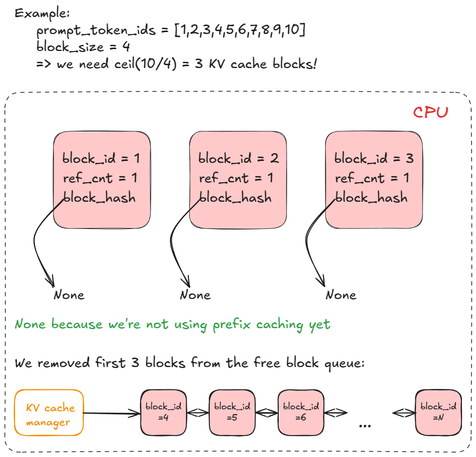
_{Figure 2. Prefix cache blocks can be shared across sequences with reference counting.^[8]}

Decode scheduling

while self.running and num_seqs < self.max_num_seqs:
    seq = self.running.popleft()
    while not self.block_manager.can_append(seq):
        if self.running:
            self.preempt(self.running.pop())
        else:
            self.preempt(seq)
            break
    else:
        num_seqs += 1
        self.block_manager.may_append(seq)
        scheduled_seqs.append(seq)
assert scheduled_seqs
self.running.extendleft(reversed(scheduled_seqs))
return scheduled_seqs, False

For decode, we don't cap max_num_batched_tokens and only consider max_num_seqs. This is because the decode phase is highly memory-bound, where every sequence has one token as input (last sampled token), so there's no risk of reaching the max number of batched tokens.

Preemption

What happens if it doesn't reach max_num_seqs but the running queue is not empty?

Since the running queue is the queue that contains all the sequences in the batch we will run on the GPU, we need to preempt sequences from the running queue back to the waiting queue.

We evict the lowest priority sequence (the last one in the running queue = the one that arrived most recently under FCFS) back to the waiting queue:

def preempt(self, seq: Sequence):
    seq.status = SequenceStatus.WAITING
    self.block_manager.deallocate(seq)
    self.waiting.appendleft(seq)

Notice we use appendleft instead of append. The scheduler puts it at the front of the waiting queue. This preserves fairness because the evicted sequence gets the highest priority to get pushed to the running queue again.

This way, the memory allocation for that sequence is freed and we get additional KV blocks to append to the sequence.

For example, let's think of a scenario where all other sequences passed can_append(seq), we have no physical blocks left in the free block queue, and two sequences (seq C: [1, 2, 3, 4, 5, 6, 8, 9, 10, 7, 12, 13], seq D: [1, 2, 3, 4, 5, 11, 8, 9, 10, 7, 14]) are left in the running queue.

The next sequence needs an additional block for the next request (currently [1, 2, 3, 4], [5, 6, 8, 9], [10, 7, 12, 13]). However, since we do not have a physical block that can be assigned, we run out of memory and can_append(seq) will return False. In this case, preemption is triggered. Since the last sequence is the only remaining sequence in the running queue, we preempt it and free three physical blocks. After that, we can successfully allocate a new block for sequence C.

Unlike prefill, decode generates one token at each forward pass, so it only checks if new block allocation is needed in the current step (if len(seq) % self.block_size == 1) instead of allocating memory in every step.

postprocess#

def postprocess(self, seqs: list[Sequence], token_ids: list[int]) -> list[bool]:
    for seq, token_id in zip(seqs, token_ids):
        seq.append_token(token_id)
        if (not seq.ignore_eos and token_id == self.eos) or seq.num_completion_tokens == seq.max_tokens:
            seq.status = SequenceStatus.FINISHED
            self.block_manager.deallocate(seq)
            self.running.remove(seq)

postprocess is the function used in LLMEngine after model_runner.call() returns the sampled token ids, which updates each sequence's state. If a sequence hits EOS or reaches max_tokens, it gets marked FINISHED, its KV blocks are deallocated (freed), and it is removed from the running queue. Freed memory becomes available for the next scheduling round.

Step 3. Actually running the Model on GPU(s)#

ModelRunner is the second part in the step() function from LLMEngine, where it is in charge of actually running the forward pass based on whatever the scheduler scheduled.

Step 3 is probably the densest(?) part of the codebase since it does distributed process management, model initialization, physical KV cache memory handling, input preparation, FlashAttention, and CUDA graph optimization. Since our primary goal is to understand the engine, we will not go deep into model and kernel-level details.

We will see

1. how model runner (and the distributed environment) is initialized.
2. how Model Runner prepares prefill and decode
3. what happens inside a forward pass (briefly)

Initializing distributed environment#

The first thing we should keep in mind is that there are $N$ ModelRunner instances created for $N$ GPUs, where rank 0 is the main process and ranks 1 to $N-1$ are all workers (recall this from the LLMEngine explanation above).

1. NCCL setup

dist.init_process_group("nccl", "tcp://localhost:2333", world_size=self.world_size, rank=rank)

• NCCL is a communication backend NVIDIA made for multiple GPUs. All processes meet at "tcp://localhost:2333".
• world_size refers to the total number of processes, which is the same as the number of GPUs used.
• dist.init_process_group lets every rank join the NCCL process group so GPU workers can communicate fast.

2. Set device / dtype / model

torch.cuda.set_device(rank)

Recall that ModelProcessor is created per world size due to the LLMEngine initialization. Rank 0 is main process and rank 1 ~ world_size - 1 are the subprocess.

torch.set_default_dtype(hf_config.torch_dtype)
torch.set_default_device("cuda")
self.model = Qwen3ForCausalLM(hf_config)

This sets the model configuration based on hf_config.

3. Load model

load_model(self.model, config.model)
self.sampler = Sampler()

When we say we "load" a model, it typically means loading the weights of the model. I found this isn't that important to understand in detail, but if interested, more explanation of load_model can be found in Appendix A. `load_model` in ModelRunner.

4. Warming up model

self.warmup_model()

If we look inside it,

def warmup_model(self):
	torch.cuda.empty_cache()
	torch.cuda.reset_peak_memory_stats()
	# ...

It first clears the cache and peak memory stats.

	max_num_batched_tokens, max_model_len = self.config.max_num_batched_tokens, self.config.max_model_len
	num_seqs = min(max_num_batched_tokens // max_model_len, self.config.max_num_seqs)
	seqs = [Sequence([0] * max_model_len) for _ in range(num_seqs)]
	self.run(seqs, True)
	torch.cuda.empty_cache()

Then it sets the worst case of the engine which we saw in the scheduling explanation (max tokens or max sequences that can be appended in one step), where it saves all the tokens and runs the sequence assuming it's prefill.

We will cover the run function in detail when we talk about how ModelRunner forward passes a batch of sequences.

5. Allocate KV cache

self.allocate_kv_cache()

Allocating KV cache (how many KV cache blocks each GPU can have in total) happens only when we initialize the ModelRunner. If interested, check Appendix B. Allocate KV Cache for detail.

6. CUDA Graph Capture

        if not self.enforce_eager:
            self.capture_cudagraph()

If enforce_eager is False, conduct CUDA Graph Capture. (Check: Eager Mode vs CUDA Graph Capture).

7. Distributed Communication (only for multiple GPU settings)

Until now, this is how all ModelRunner instances are initialized, and this part is where the main process and its workers diverge.

		if self.world_size > 1:
            if rank == 0:
                self.shm = SharedMemory(name="nanovllm", create=True, size=2**20)
                dist.barrier()
            else:
                dist.barrier()
                self.shm = SharedMemory(name="nanovllm")
                self.loop()

For rank 0, the main model runner creates Shared Memory, which is used to communicate which sequences to process.

After the main model runner creates Shared Memory, each rank's model runner connects to the Shared Memory and waits for the Main Model Runner's instructions.

Preparing Prefill and Decode#

So how does "execute a forward pass" actually work under the hood after initializing the Model Runner?

In the step() function from LLMEngine, the entry point for model runner is this line:

token_ids = self.model_runner.call("run", seqs, is_prefill)

This calls the run function in Model Runner. run function is where the actual forward pass (inference) happens.

    def run(self, seqs: list[Sequence], is_prefill: bool) -> list[int]:
        input_ids, positions = self.prepare_prefill(seqs) if is_prefill else self.prepare_decode(seqs)
        temperatures = self.prepare_sample(seqs) if self.rank == 0 else None
        logits = self.run_model(input_ids, positions, is_prefill)
        token_ids = self.sampler(logits, temperatures).tolist() if self.rank == 0 else None
        reset_context()
        return token_ids

Prepare Prefill

Let's first look at the scenario where all scheduled sequences are in prefill.

prepare_prefill() has to turn a list of Sequence objects into the flat tensors expected by the model and FlashAttention. The core loop looks like this:

for seq in seqs:
    start = seq.num_cached_tokens
    seqlen_q = seq.num_scheduled_tokens
    end = start + seqlen_q
    seqlen_k = end
    input_ids.extend(seq[start:end])
    positions.extend(range(start, end))
    cu_seqlens_q.append(cu_seqlens_q[-1] + seqlen_q)
    cu_seqlens_k.append(cu_seqlens_k[-1] + seqlen_k)

For each sequence, there are four local values:

• start: the first token position that needs to be computed. If there is no prefix cache, start = 0. If the first four tokens are already cached, start = 4.
• end: the exclusive end position of the chunk being computed, so the actual input slice is seq[start:end].
• seqlen_q: the number of query tokens computed in this forward pass. In prefill, this is the scheduled prompt chunk length. If there is prefix cache that can be reused, this may be only the uncached suffix.
• seqlen_k: the full key/value context length visible to attention. It equals end, because the newly computed query tokens can attend to every token from position 0 up to end - 1.

Then two different kinds of tensors are built.

First, input_ids and positions describe the actual tokens this forward pass will compute:

input_ids.extend(seq[start:end])
positions.extend(range(start, end))

Second, cu_seqlens_q and cu_seqlens_k describe where each sequence begins and ends inside the flattened attention batch:

cu_seqlens_q.append(cu_seqlens_q[-1] + seqlen_q)
cu_seqlens_k.append(cu_seqlens_k[-1] + seqlen_k)

positions are used by the model's positional logic (e.g. RoPE), while cu_seqlens_q and cu_seqlens_k are what FlashAttention uses to recover per-sequence boundaries (needed in Attention) from the flat batch.

The remaining part of prepare_prefill() computes where the newly generated K/V vectors should be written in the physical KV cache:

start_block = start // self.block_size
end_block = (end + self.block_size - 1) // self.block_size
for i in range(start_block, end_block):
    slot_start = seq.block_table[i] * self.block_size
    if i == start_block:
        slot_start += start % self.block_size
    # ...
    slot_mapping.extend(range(slot_start, slot_end))

It uses seq.block_table to translate logical block positions into physical KV cache block slots. This is also passed as Context, used during Attention operation.

If prefix cache is enabled (cu_seqlens_k[-1] > cu_seqlens_q[-1]), we need to load the KV cache that we are going to reuse. prepare_prefill() prepares block_tables, which are the lists of physical KV blocks mapped to each sequence, so FlashAttention can read cached prefix K/V from the KV cache.

Finally, set_context(...) stores all of this metadata inside the GPU device so the attention layer can run with the correct batch layout.

Now let's walk through an example where a single batch includes one sequence that uses prefix cache and one sequence that is a fresh prompt.

Assume a situation where Sequence A has already been processed:

seq_a = [1, 2, 3, 4, 5, 6, 7]
# "Write a travel plan for Seoul."

Only the first full block can be reused:

cached full block: [1, 2, 3, 4]  # "Write a travel plan"
not reused as a block: [5, 6, 7] # "for Seoul."

Now the next prefill batch contains two sequences:

seq_c = [1, 2, 3, 4, 5, 6, 7, 8, 9, 10]
# "Write a travel plan for Seoul. Include traditional markets"

seq_e = [21, 22, 23, 24, 25]
# "The capital of France is"

seq_c reuses its first full block, while seq_e is new:

seq_c.num_cached_tokens = 4
seq_c.num_scheduled_tokens = 6

seq_e.num_cached_tokens = 0
seq_e.num_scheduled_tokens = 5

For seq_c, the local prefill values are:

start = 4
seqlen_q = 6
end = 10
seqlen_k = 10

We can see that seqlen_q is shorter than seqlen_k due to prefix cache. seq_c contributes only its uncached suffix of length 6 to the model input:

input_ids += [5, 6, 7, 8, 9, 10]
positions += [4, 5, 6, 7, 8, 9]

For seq_e, there is no prefix cache so seq_e contributes its entire prompt:

input_ids += [21, 22, 23, 24, 25]
positions += [0, 1, 2, 3, 4]

After both sequences are processed, the flattened batch becomes:

input_ids = [
    5, 6, 7, 8, 9, 10,
    21, 22, 23, 24, 25,
]

positions = [
    4, 5, 6, 7, 8, 9,
    0, 1, 2, 3, 4,
]

The cumulative lengths of the batch are:

cu_seqlens_q = [0, 6, 11]
cu_seqlens_k = [0, 10, 15]

where cu_seqlens_q is the boundary of flattened query rows and cu_seqlens_k is the boundary in the full key/value context.

Prepare Decode

Compared to prepare_prefill(), prepare_decode() is much simpler. Every sequence contributes exactly one token because decode only ever needs to process the most recently sampled token:

def prepare_decode(self, seqs: list[Sequence]):
    input_ids = []
    positions = []
    slot_mapping = []
    context_lens = []
    for seq in seqs:
        input_ids.append(seq.last_token)
        positions.append(len(seq) - 1)
        context_lens.append(len(seq))
        slot_mapping.append(seq.block_table[-1] * self.block_size + (len(seq) - 1) % self.block_size)
    # ...

Going back to our running example: suppose seq_a = [1, 2, 3, 4, 5, 6, 7] just finished prefill and sampled token 8.

For the next decode step:

input_ids = [8]
positions = [7]

and the slot for the new token is computed from the last block (seq.block_table[-1]) in seq.block_table, offset by where we are inside that block.

Because every sequence contributes just one token, there's no need to bookkeep cumulative sequence lengths (cu_seqlens_q / cu_seqlens_k) as we did in prefill. Decode's batch is just num_seqs tokens, one per row.

Executing forward pass for each given batch#

For a prefill request, we conduct the forward pass by return self.model.compute_logits(self.model(input_ids, positions))

This one line consists of the full forward pass of the Transformer (Qwen) Architecture.

which largely is input_ids -> VocabParallelEmbedding -> [Attention -> RMSNorm -> MLP] x N -> final RMSNorm -> ParallelLMHead -> Sampler

We will not go into all the details of the Transformer internals since there are already many great resources^[9] that cover this in depth. We will mainly look inside how Attention and KV Cache is used.

Attention in nano-vLLM#

def forward(self, q: torch.Tensor, k: torch.Tensor, v: torch.Tensor):

In the $n$'th layer of the Decoder, we receive these shapes as inputs:

q: [num_tokens, num_q_heads, head_dim]
k: [num_tokens, num_kv_heads, head_dim]
v: [num_tokens, num_kv_heads, head_dim]

Then we get the batch metadata (Context) from Model Runner.

if k_cache.numel() and v_cache.numel():
	store_kvcache(k, v, k_cache, v_cache, context.slot_mapping)

This line (if k_cache.numel() and v_cache.numel():) checks whether KV cache tensors are real allocated tensors from the earlier QKV linear projection. When Model Runner is warming up, this is skipped. If this is true, we store the KV cache using store_kv_cache().

Then the store_kv_cache() function launches a triton kernel as follows:

store_kvcache_kernel[(N,)](key, key.stride(0), value, value.stride(0), k_cache, v_cache, slot_mapping, D)

where

• N: One Triton program is launched per token's KV cache.
• key, value: fresh key / value tensor from the current attention forward pass.
• key.stride(0),value.stride(0): memory distance between key[idx]/value[idx] and key[idx + 1]/value[idx + 1]. Used to find each token row’s key vector.
• k_cache, v_cache: persistent key/value cache tensor where new keys are written (which will be retrieved for later forward passes)
• slot_mapping: maps each current token row to a physical KV cache slot.
• D: flattened const size of one token’s K/V vector - num_kv_heads * head_dim.

@triton.jit
def store_kvcache_kernel(
    key_ptr,
    key_stride,
    value_ptr,
    value_stride,
    k_cache_ptr,
    v_cache_ptr,
    slot_mapping_ptr,
    D: tl.constexpr,
):
    idx = tl.program_id(0)
    slot = tl.load(slot_mapping_ptr + idx)
    if slot == -1: return
    key_offsets = idx * key_stride + tl.arange(0, D)
    value_offsets = idx * value_stride + tl.arange(0, D)
    key = tl.load(key_ptr + key_offsets) # shape [D,]
    value = tl.load(value_ptr + value_offsets) # shape [D,]
    cache_offsets = slot * D + tl.arange(0, D)
    tl.store(k_cache_ptr + cache_offsets, key)
    tl.store(v_cache_ptr + cache_offsets, value)

We want to store the fresh K, V cache from the current forward pass to persistent physical KV cache memory. store_kvcache_kernel programs are launched where one program saves (tl.store) one token's KV to a physical KV cache slot.

After that, we process FlashAttention to prefill or decode Sequences.

if context.is_prefill:
	if context.block_tables is not None:    # prefix cache
		k, v = k_cache, v_cache
	o = flash_attn_varlen_func(q, k, v,
							   max_seqlen_q=context.max_seqlen_q, cu_seqlens_q=context.cu_seqlens_q,
							   max_seqlen_k=context.max_seqlen_k, cu_seqlens_k=context.cu_seqlens_k,
							   softmax_scale=self.scale, causal=True, block_table=context.block_tables)
	else:    # decode
		o = flash_attn_with_kvcache(q.unsqueeze(1), k_cache, v_cache,
									cache_seqlens=context.context_lens, block_table=context.block_tables, 
									softmax_scale=self.scale, causal=True)

Eager Mode vs CUDA Graph Capture#

While prefill always uses self.model.compute_logits(self.model(input_ids, positions)) for forward pass, we may sometimes use what is called CUDA Graph Capture mode.

Before we look into the codebase, what is eager mode and CUDA graph capture?

Eager mode means PyTorch executes operations immediately, one by one, as normal Python code runs. So self.model.compute_logits(self.model(input_ids, positions)) will launch: embedding kernel, attention kernels, linear kernels, norm kernels, MLP kernels, LM head kernel, etc. in a dynamic manner, for every forward pass. While this is flexible, it creates overhead from calling Python/PyTorch to launch kernels every time.

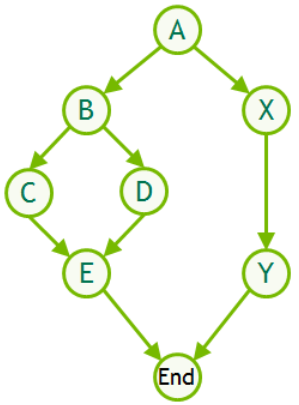
_{Figure 3. CUDA Graph capture records a stable sequence of GPU operations for replay.}

CUDA Graph (Capture) is an optimization where we first run the model once, record the exact sequence of CUDA operations, and then replay that recorded graph later.

So instead of asking PyTorch to rebuild and launch every kernel step by step every decode iteration, CUDA graph replay runs the same captured GPU work again with new input data. This is possible because the model pipeline is usually stable. This reduces CPU launch overhead.

However CUDA graphs are much less flexible. The captured graph expects stable tensor shapes and memory addresses.

In nano-vLLM, that is why nano-vLLM uses it only for scenarios that satisfy the below requirements:

• batch is decode and
• eager mode is False and
• size of input ids (input tokens) is smaller than 512.

if is_prefill or self.enforce_eager or input_ids.size(0) > 512:
    return self.model.compute_logits(self.model(input_ids, positions))
else:
    ...
    graph.replay()
    return self.model.compute_logits graph_vars["outputs"][:bs]

It is hard to use CUDA graph capture in prefill because prompt length, total tokens, and attention shapes are highly variable. This makes efficient graph capture very hard.

Wrapping Up#

We started from example.py and went all the way down to the model’s forward pass.

In the end, an LLM inference engine is mostly this loop:

1. Scheduler picks which sequences to run,
2. Block Manager ensures their KV cache blocks are ready,
3. Model Runner builds a compact batch,
4. Runs the model,
5. Appends the new tokens and updates the sequences.

with additional nuances (engineering) to make the loop efficient under memory constraints. Hope this note helped you understand the engine better, and I will come back with other interesting write-ups.

Appendix#

Appendix A. load_model in ModelRunner#

According to utils.py, load_model is as follows:

def load_model(model: nn.Module, path: str):
    packed_modules_mapping = getattr(model, "packed_modules_mapping", {})
    for file in glob(os.path.join(path, "*.safetensors")):
        with safe_open(file, "pt", "cpu") as f:
            for weight_name in f.keys():
                for k in packed_modules_mapping:
                    if k in weight_name:
                        v, shard_id = packed_modules_mapping[k]
                        param_name = weight_name.replace(k, v)
                        param = model.get_parameter(param_name)
                        weight_loader = getattr(param, "weight_loader")
                        weight_loader(param, f.get_tensor(weight_name), shard_id)
                        break
                else:
                    param = model.get_parameter(weight_name)
                    weight_loader = getattr(param, "weight_loader", default_weight_loader)
                    weight_loader(param, f.get_tensor(weight_name))

In optimized inference engines like vLLM, models may define packed_modules_mapping to fuse separate weights (e.g., q, k, v) into a single tensor.

For example, if the QKV projection weight is saved as:

{  
"q_proj": ("qkv_proj", "q"),  
"k_proj": ("qkv_proj", "k"),  
"v_proj": ("qkv_proj", "v"),  
}

for k in packed_modules_mapping:
	if k in weight_name:
		v, shard_id = packed_modules_mapping[k]
		param_name = weight_name.replace(k, v)
		param = model.get_parameter(param_name)
		weight_loader = getattr(param, "weight_loader")
		weight_loader(param, f.get_tensor(weight_name), shard_id)
		break

If a weight corresponds to a packed module, this part remaps it and loads it into the correct shard of the fused parameter (e.g. q_proj -> qkv_proj[0] ...)

Appendix B. Allocate KV Cache in Model Runner#

According to the vLLM-omni documentation^[10], a useful formula for memory calculation is to calculate the total available VRAM - model weight memory - activation memory.

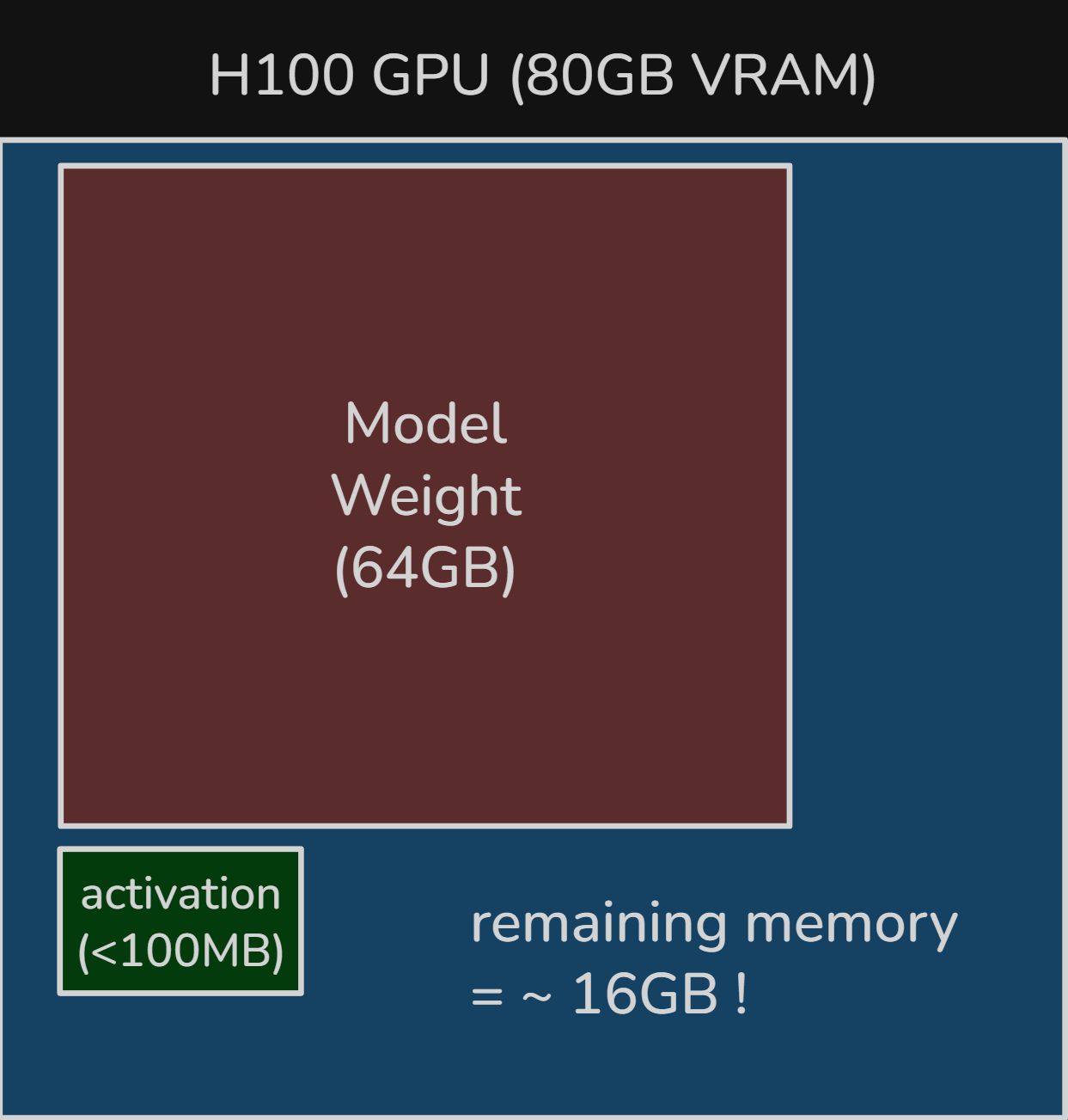
_{Figure 4. Example of remaining VRAM headroom after loading about 64 GB of model weights: roughly 16 GB for KV cache, activations, workspace buffers, and runtime overhead.^[11][12]}

That's the amount of memory we can use for KV cache.

Now we will look at the code:

def allocate_kv_cache(self):
	# ...
	free, total = torch.cuda.mem_get_info()
	used = total - free

We check the total memory and free memory and calculate how much memory is used "currently". This includes model weights and activation memory, while also other minor overheads such as CUDA runtime overhead or GPU memory used by other processes.

	peak = torch.cuda.memory_stats()["allocated_bytes.all.peak"]
	current = torch.cuda.memory_stats()["allocated_bytes.all.current"]

This part is to get the activation memory. While activation memory can be a bottleneck during training, in inference, this is ephemeral memory that is only reserved for a single step. By using CUDA's API, we reserve this space by checking the "worst case" (peak activation memory) during the dummy forward pass we did.

	num_kv_heads = hf_config.num_key_value_heads // self.world_size

It is important to keep in mind that each GPU rank has its own Model Runner instance. So if we are using multiple GPUs with Tensor Parallelism, each GPU processes its own part of the whole job simultaneously.

Tensor Parallelism is a method where we shard the tensor of each layer, and GPU ranks process each subpart. During Attention, the tensor is sharded by the number of KV heads, which differ based on which Attention mechanism is used.

For example, if the model uses standard MHA(Multi-Head Attention), KV heads will be the size of heads. If it uses GQA(Grouped-Query Attention), KV heads will be the size of heads/group size.

	head_dim = getattr(hf_config, "head_dim", hf_config.hidden_size // hf_config.num_attention_heads)
	block_bytes = 2 * hf_config.num_hidden_layers * self.block_size * num_kv_heads * head_dim * hf_config.torch_dtype.itemsize

KV Cache is a per-token per-layer cache that saves the K and V values of processed tokens. This can be saved and reused because KV Cache is only dependent on past tokens and doesn't change based on future tokens.

Then what's the actual shape of KV cache in memory bytes?

It is [2, num_layers, num_blocks, block_size, num_kv_heads, head_dim, dtype]

where

• 2: for K and V
• num_layers: because KV cache is per layer
• block size: PagedAttention allocates memory based on block size
• number of KV heads: KV cache shape per token is `(num_kv_heads, head_dim)
• head dimension: KV cache shape per token is (num_kv_heads, head_dim)
• data type: int4 = 0.5 byte, fp8 = 1 byte, fp16 = 2 byte etc.

	config.num_kvcache_blocks = int(total * config.gpu_memory_utilization - used - peak + current) // block_bytes
	assert config.num_kvcache_blocks > 0
	self.kv_cache = torch.empty(2, hf_config.num_hidden_layers, config.num_kvcache_blocks, self.block_size, num_kv_heads, head_dim)

Calculates the total KV cache blocks that we can assign given the GPU memory utilization configuration.

	layer_id = 0
	for module in self.model.modules():
		if hasattr(module, "k_cache") and hasattr(module, "v_cache"):
			module.k_cache = self.kv_cache[0, layer_id]
			module.v_cache = self.kv_cache[1, layer_id]
			layer_id += 1

Finally, assign KV slots (actual tensor storage in GPU) for each layer of the model's Attention layers.

References#

1. nano-vLLM repository: https://github.com/GeeeekExplorer/nano-vLLM
2. Previous post on what inference engines optimize: https://github.com/junuxyz/mlsys-notes/blob/main/notes/llm-inference-intro-p1.md#what-inference-engine-optimizes
3. Sebastian Raschka, "Coding the KV Cache in LLMs": https://magazine.sebastianraschka.com/p/coding-the-kv-cache-in-llms
4. Hugging Face KV cache blog: https://huggingface.co/blog/kv-cache
5. PagedAttention note: https://github.com/junuxyz/mlsys-notes/blob/main/notes/pagedattention.md
6. FIFO / FCFS background: https://en.wikipedia.org/wiki/FIFO_(computing_and_electronics)
7. Minimal prefix hash experiment: https://gist.github.com/junuxyz/89501be9327da5e137515874d4c5b8e1
8. Aleksa Gordic, "vLLM": https://www.aleksagordic.com/blog/vllm
9. The Annotated Transformer: https://nlp.seas.harvard.edu/annotated-transformer/
10. vLLM-omni GPU memory utilization documentation: https://docs.vllm.ai/projects/vllm-omni/en/latest/configuration/gpu_memory_utilization/#useful-formula-for-memory-calculation
11. VRAM headroom figure source: https://github.com/junuxyz/mlsys-notes/blob/main/assets/notes/llm-inference-intro-p1/llm-inference-intro-p1-15.png
12. Memory needed to decode explanation: https://github.com/junuxyz/mlsys-notes/blob/main/notes/llm-inference-intro-p1.md#how-much-memory-is-needed-to-decode