Sarathi-Serve paper review

Table of contents

• TL;DR
• Background
  • Takeaway 1
  • Takeaway 2
  • What is SLO?
  • The effect of mixed batching
  • Takeaway 3
  • Pipeline Parallelism
  • Pipeline Bubbles
  • Takeaway 4
• Sarathi-Serve
  • Chunked Prefill
  • Overhead
  • Stall Free Batching
  • Stall Free Batching w/ Illustrated Example
• How Sarathi-Serve solves the problem
  • Considerations (Tradeoffs) for determining token budget
• Notes on evaluation
• Code Example: nano-vLLM-v1
• References

TL;DR#

To explain Sarathi-Serve in one sentence, it introduces a way to overcome generation stalls from decode requests by implementing chunked prefill and stall-free batching.

We will talk more about what this means later.

While the field seems to favor optimizing prefill and decode separately (P/D disaggregation), the ideas introduced in this paper^[1] are still widely used in industry standard inference engines such as vLLM or SGLang (especially for single node cases).

Background#

In the background section, I will mainly talk about four takeaways, following the paper's narrative.

I will not talk about batching, since I've already explained it in my previous notes.^[11][12]

One thing to note is that batching works especially well for decode requests rather than prefill requests. This is because if the input is long enough, just one prefill request can saturate the GPU and make it compute-bound. Since it is already compute-bound, there is no merit in adding batches.

On the other hand, decode is usually memory-bound, so throughput scales linearly when requests are batched together. Again, I talked about this in Introduction to LLM Inference Part 1.^[12], so I will not repeat myself.

The figure in the paper shows this:

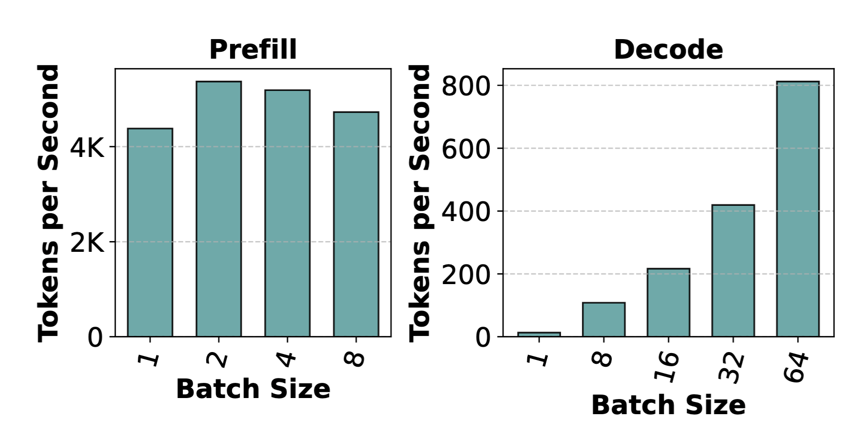
_{Figure 1. Batching improves decode throughput much more than prefill throughput.^[1]}

So the first takeaway is:

Takeaway 1#

The two phases of LLM inference, prefill and decode, demonstrate contrasting behaviors wherein batching boosts decode phase throughput immensely but has little effect on prefill throughput.

Now let's talk about how to measure total execution time in LLM inference. More generally, for any program that does something repetitively, execution is either bound by the time spent computing the data or by the time spent loading and storing it in memory.

We can express this as $T = \max(T_{\text{math}}, T_{\text{mem}})$.

How can we ignore the non-dominant time cost? We will look at this with a simple example, borrowing Horace He's aesthetic image^[2]:

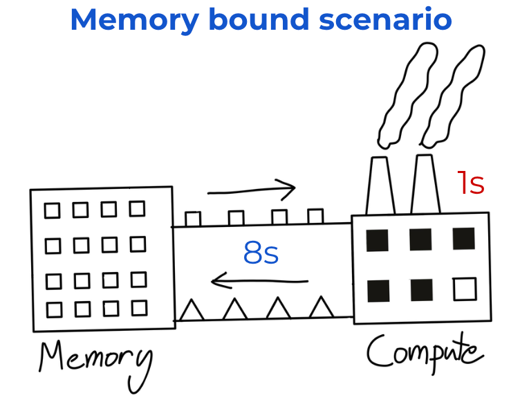
_{Figure 2. A memory-bound workload where memory transfer dominates compute for a single request.^[2]}

Suppose we have a memory-bound scenario (which resembles a decode scenario) with low arithmetic intensity.^[12] Computing the data takes only one second, while retrieving and rewriting the data takes 8 seconds.

If we run only one workload on such a program, the total time would be 1 + 8 = 9 seconds.

However, suppose we have more than 1,000 workloads repeating the same thing.

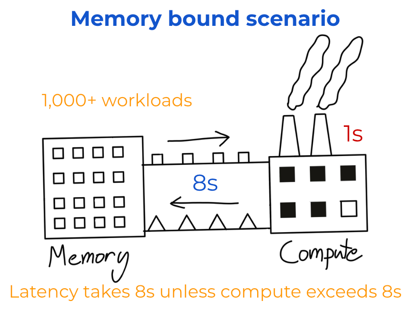
_{Figure 3. Repeated memory-bound workloads hide compute time and remain dominated by memory access.^[2]}

When the first batch of data goes in, compute is done after a second, and then it stays idle for 7 seconds until the next batch of data comes in. So if multiple workloads are continuously executed, the 1s cost of compute gets hidden and the system is bound by the dominant time (in this case, $T_{\text{mem}}$) until $T_{\text{math}}$ exceeds 8 seconds.

This is why $T$ can be expressed as $\max(T_{\text{mem}}, T_{\text{math}})$.

This also means that, theoretically, increasing the smaller cost adds no extra end-to-end latency until it reaches the dominant cost.

Takeaway 2#

So the second takeaway we have is:

Decode batches operate in a memory-bound regime leaving compute underutilized.

This implies that more tokens can be processed along with a decode batch without significantly increasing its latency.

Now we will review earlier inference engines: FasterTransformer, Orca, and vLLM (v0). We will first compare FasterTransformer and vLLM v0, and then talk about Orca.

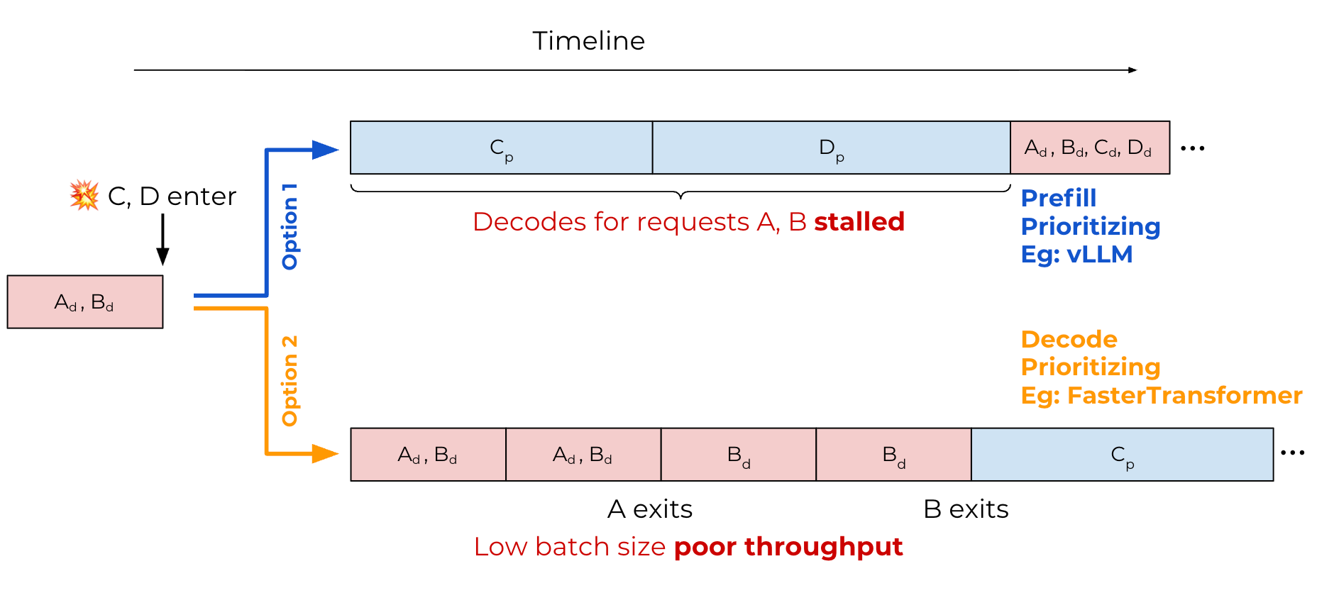
_{Figure 4. vLLM v0 and FasterTransformer compared as prefill-prioritizing and decode-prioritizing schedulers.^[3]}

vLLM v0 (Option 1 in the image above) is prefill-prioritizing and eagerly admits prefills before resuming ongoing decodes. As seen in the image, even if a new request comes in, it prioritizes the new request's prefill over the earlier requests' decode steps. This leads to high throughput because we can batch more decode steps after every request is in the decode phase, but it also leads to higher TPOT.

In the image, A and B need to wait for C_p and D_p to finish processing. This is called generation stalls, which I mentioned in the tl;dr.

FasterTransformer (Option 2) used static batching, which takes a request batch, runs prefill and decode steps on it until all the requests are finished processing, then executes the next request batch in the same manner.

This can be called a decode-prioritizing system, since it prioritizes decode steps instead of adding new prefills to increase throughput. This leads to low TPOT, but overall throughput is also low.

Orca was the only engine back then that supported mixed (hybrid) batching (in early 2024).

Orca introduced selective batching, which batches all non-attention operations and runs attention per request only (since attention should be applied per request). For an in-depth explanation, check out Improving LLM Inference with Continuous Batching: Orca through tinyorca.^[11]

However, Orca's hybrid batching did not turn out to be optimal because it increased latency, which often exceeded the SLO.

What is SLO?#

SLO stands for Service Level Objective, which refers to a target performance level for a particular metric. This sets a standard for what is considered acceptable service that does not harm user experience.^[4]

Usually, in the context of LLM inference, this boils down to metrics such as TPOT and TTFT. Throughout this post, let's assume TPOT must be <10ms.

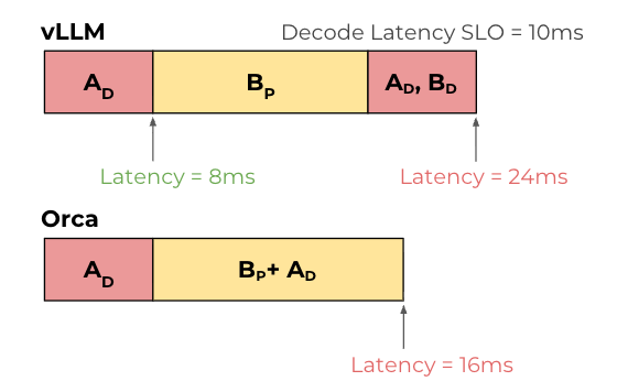
_{Figure 6. Both vLLM and Orca exceed the decode latency SLO under mixed batching.^[3]}

Above is an image showing that both vLLM and Orca do not satisfy the latency SLO (10ms). We already saw why this happens in vLLM (it prioritizes prefill requests first). But you can see that Orca's hybrid batching increases latency in a fairly subtle manner.

The effect of mixed batching#

Hybrid batching works as follows:

1. Run token-wise operations (LayerNorm, QKV projection, MLP) on a flattened batch: [sum_i S_i, hidden]
2. Split into per-request tensors when execution reaches the attention path, where request i is [S_i, hidden]
3. Run the request-local attention path independently per request.
4. Re-flatten the outputs into a single token stream.
5. Continue with token-wise operations and repeat for the next layer.

In a hybrid iteration, decode-side attention work may finish earlier than the larger prefill-side attention work, but decode requests still wait for the completion of the entire hybrid iteration before their next token can be returned.^[5][6]

Although prefill remains the dominant part of the hybrid iteration, the latency can slightly exceed that of a standalone prefill (as seen in the image above; 8ms vs 9ms) because the batch also includes decode-side work and incurs additional hybrid-batching overhead, such as batch formation and split/merge-related^[7] execution overhead.

So the step time for hybrid batching comes from $T_{\text{hybrid}} \approx T_{\text{batched non-attention}} + T_{\text{attention related operation for requests}} + T_{\text{overhead}}$.

Note: The attention-related term is not directly observable as a single per-request quantity; it emerges from the combined execution of the hybrid batch.

Takeaway 3#

The third takeaway the authors mentioned is that the interleaving of prefills and decodes involves a trade-off between throughput and latency for current LLM inference schedulers.

State-of-the-art systems (like vLLM v0) use prefill-prioritizing schedules, which improve throughput but also have side effects, most notably generation stalls.

Another takeaway I want to explicitly mention (while already explained implicitly) is that not all step sizes are the same. Decode steps finish much more quickly, prefill steps take longer, and a hybrid batch of them takes even longer than that due to overhead.

Pipeline Parallelism#

Pipeline parallelism (PP) is a method where we shard the model weights vertically, dividing them into groups of layers. For example, if we use four GPUs for PP with a model that has 80 layers, each device will take 20 layers (e.g., device 0 gets layers 0-19, device 1 gets layers 20-39, ...). Unlike training, we do not need a backward pass for inference, so it is an even better fit for inference than for training.

So if we apply this to a forward pass scenario, GPU 0 processes the first 20 layers and sends data to GPU 1 and GPU 1 processes the next 20 layers, and so on.

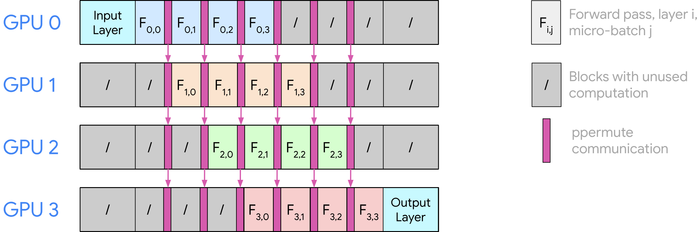
_{Figure 7. Pipeline parallelism splits layers across devices so one micro-batch flows stage by stage.^[8]}

For more in-depth explanation on PP, I recommend these two articles.^[9][10]

Pipeline Bubbles#

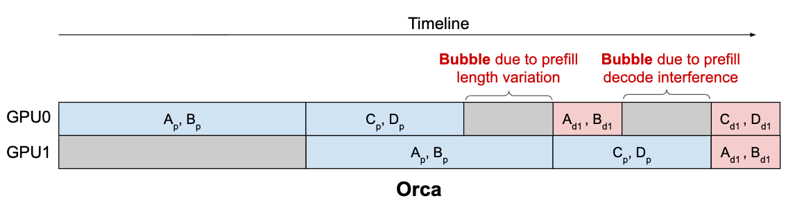
_{Figure 8. Uneven iteration times create pipeline bubbles where some devices wait idly.^[1]}

Another problem that appears when using multiple GPUs in Orca is pipeline bubbles.

In Takeaway 3, I already mentioned that step sizes are not the same. Since the size of each step has high variance, performance is bound by the longest processing time among the GPUs at that moment.

For example, in the image above, GPU0 finishes processing the prefills for C and D while GPU1 is still processing the prefills for A and B, whose inputs are longer and therefore take more time. GPU0 has to wait until GPU1 is finished before it can pass data along. This gets even worse when GPU1 is processing prefill while GPU0 has already finished processing decode, which ends earlier.

Takeaway 4#

Again, step sizes are NOT the same. This can lead to large variance in the compute time of LLM iterations, depending on the composition of prefill and decode tokens in the batch. This introduces significant bubbles when using pipeline parallelism.

Sarathi-Serve#

If we add up all the insights from the four takeaways (especially Takeaway 2), we can think of making hybrid batching "smarter" by carefully adding prefill computation. This will introduce little to no additional cost while increasing throughput.

To do this, Sarathi-Serve introduces chunked prefill and stall-free batching with a token budget.

Chunked Prefill#

Chunked prefill is a technique used in stall-free batching that allows "partial" prefill. Before this paper, prefill was processed atomically: either all or none.

By using chunked prefill, we can process only part of it per step. This gives us flexibility in how much we process in one step. We will talk more about this in stall-free batching.

Overhead#

Chunked prefill introduces additional overhead compared to standard prefill. In a regular prefill, all input tokens are processed in a single pass, so there is no need to revisit previously computed KV states.

With chunked prefill, however, the prefill phase is split across multiple iterations. Each new chunk must attend to tokens from earlier chunks, which requires repeatedly reading the previously computed KV cache during attention.

This results in extra memory reads due to KV cache re-access.

In practice, this overhead remains modest because prefill is largely compute-bound, so the additional KV reads have limited impact on overall runtime. According to the ablation study section, the overhead is at most around 25% for small chunk sizes and becomes negligible for larger chunks.

Stall Free Batching#

This is the scheduling algorithm introduced in Sarathi-Serve:

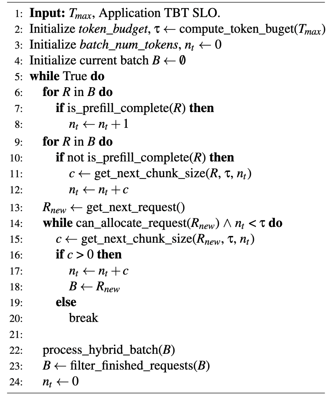
_{Figure 12. Sarathi-Serve's stall-free batching algorithm uses a fixed token budget for each step.^[1]}

If we break down the algorithm, stall-free batching works as follows:

1. Initialize a token budget.

   Token budget is the fundamental knob used in Sarathi-Serve, which determines how many tokens to allow in a step. This is static throughout serving. We will talk more about the considerations and tradeoffs involved in setting the token budget.

2. Also initialize batch number of tokens.

   This is used to check whether the current batch has exceeded the token budget.

3. For each step:

   1. Prefer decode requests first.

   2. Update the batch number of tokens and the remaining token budget.

   3. Check whether there is a partially processed prefill request with tokens remaining.

      If yes:

      • Set the chunk size to min(remaining budget, remaining prefill length).
      • If the remaining budget is 0, end this step.
      • Otherwise, continue to the next sub-step.

   4. Update the batch number of tokens and the remaining token budget again.

   5. Get the next request and repeat the same logic until the token budget for this step is exhausted.

4. Process hybrid batching of all the requests selected in step 3.

To make this more concrete, I will walk through an illustrated example that hopefully makes the scheduling process more intuitive.

Stall Free Batching w/ Illustrated Example#

Suppose we have a token budget of 100.

With 4 requests R1~R4 in their decode phase, one chunked request (from an earlier step) R5(30 tokens), and two prefill requests R6(80 tokens) and R7(150 tokens):

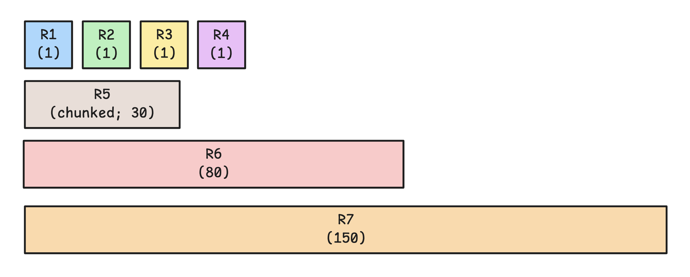
batch_num_tokens is initialized to 0 for each step.

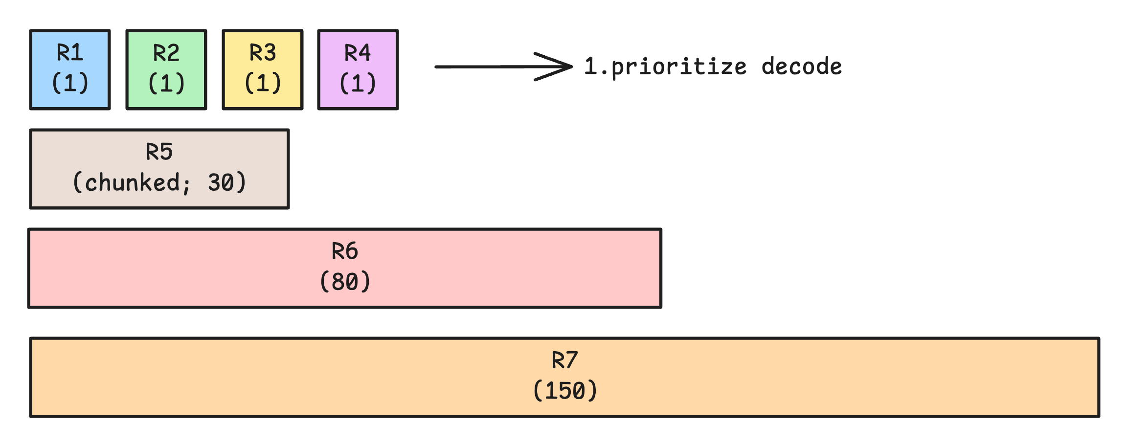
First, we need to process all four decode requests, so we schedule them. batch_num_tokens becomes 4.

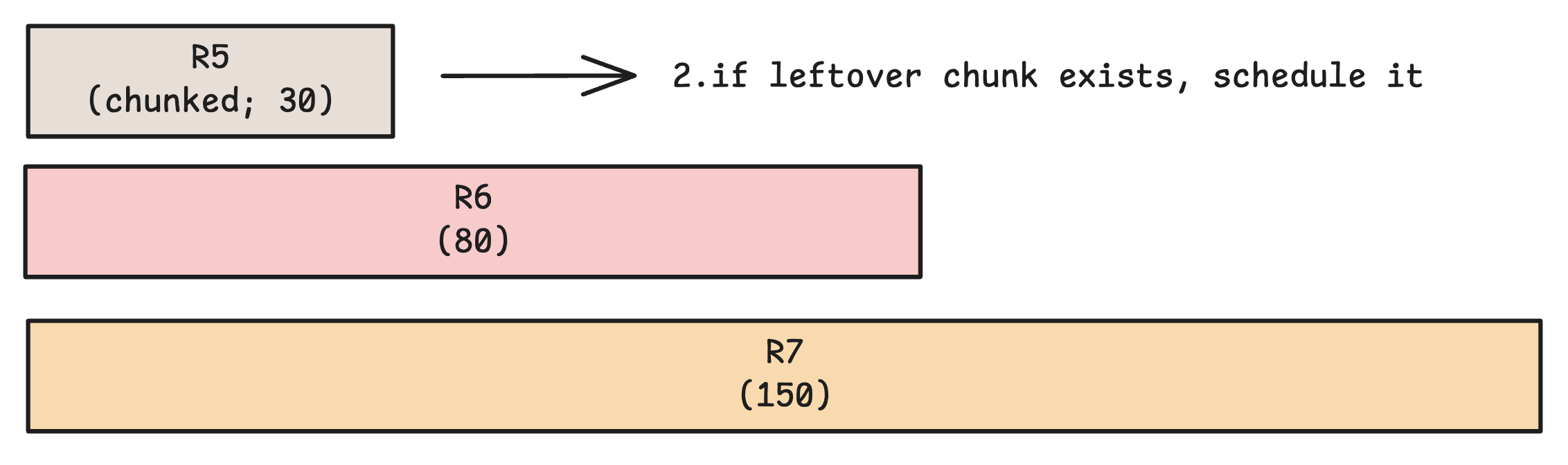
Since batch_num_tokens (4) did not reach the token budget (100), we continue.

We prioritize the chunked request, which is R5 in this case. min(remaining_budget, R5) = 30, so we schedule it to process the whole leftover prefill request. batch_num_tokens is updated to 34.

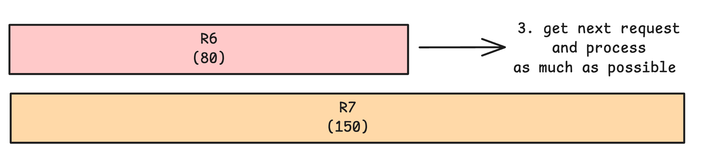
The next request (in FCFS order) is R6, so we determine how much of it we can schedule. It turns out that min(remaining_budget, R6) = 66, so we chunk R6 and schedule only its first 66 tokens.

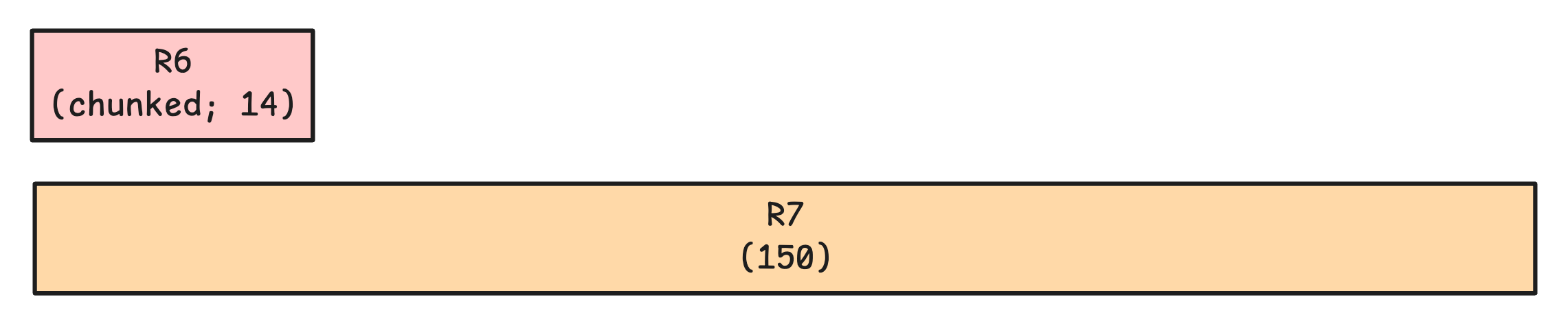
The remainder stays pending for future iterations.

So R1 ~ (chunked) R6 are scheduled for this step and processed in hybrid batch.

For this iteration, the step latency can be approximated as $T_{\text{hybrid}} \approx T_{\text{batched non-attention}} + T_{\text{attention related operation for requests}} + T_{\text{overhead}}$

How Sarathi-Serve solves the problem#

Stall-free batching does use the hybrid batching technique introduced by Orca, but the difference is that instead of using the number of requests as an upper bound, it uses a token budget.

Before Sarathi-Serve, batched tokens per step had high variance because some steps batch together long prefills, while other steps consist mostly of decodes. Also, request input lengths differ, so some batched prefills take a very long time.

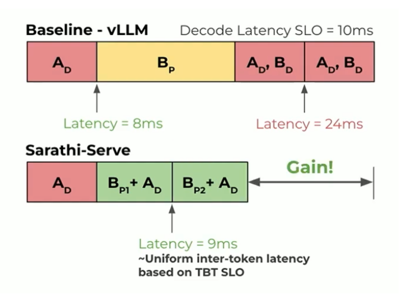
_{Figure 19. Without a token budget, per-step work varies widely depending on the batch mix.^[3]}

By capping the token budget, we can control and estimate worst-case step latency much better, since it is bounded by a batch whose total tokens are approximately equal to the token budget. The token budget is usually capped to match the SLO requirement (e.g., < 10ms), so we can batch more prefill tokens while adding minimal latency to the decode steps batched with them.

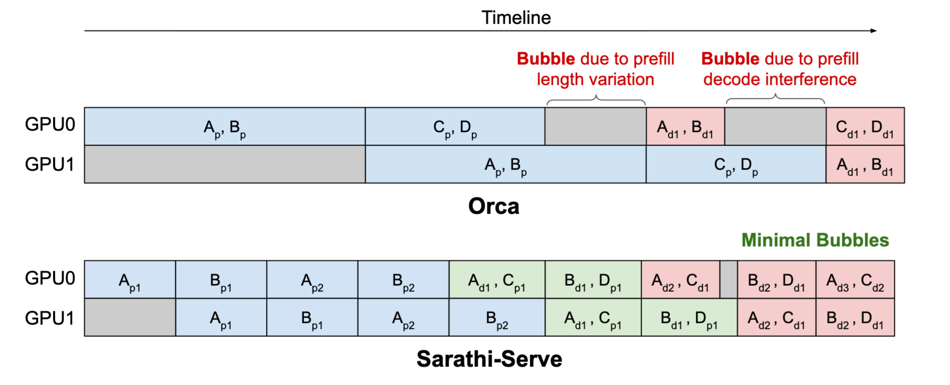
_{Figure 20. A token budget bounds step latency and reduces variance across iterations.^[1]}

Also, since each step is capped to the token budget, variance becomes much lower, minimizing the pipeline bubbles.

Considerations (Tradeoffs) for determining token budget#

Choosing the token budget is a tradeoff among latency, efficiency, and hardware behavior.

1. TBT(TPOT) SLO (primary constraint)

   Since the point of having a token budget is to satisfy the decode SLOs, the budget must be small enough to avoid exceeding the requirement. If too many prefill tokens are included, decode iterations get delayed, causing generation stalls.

2. Tile Quantization

   GPU kernels operate on fixed tile sizes (e.g., 16×16, 32×32). Misaligned chunk sizes can lead to wasted computation. For example, a chunk size of 257 can increase prefill time by ~32% due to poor tiling efficiency. (tbh I don't know how they manage to make this efficient because of my understanding, token budget only caps the upper bound)

3. Pipeline Bubbles

   Larger chunks increase variation in iteration time, which leads to pipeline bubbles in pipeline-parallel setups. Smaller, more uniform chunks help maintain balanced execution across stages.

Notes on evaluation#

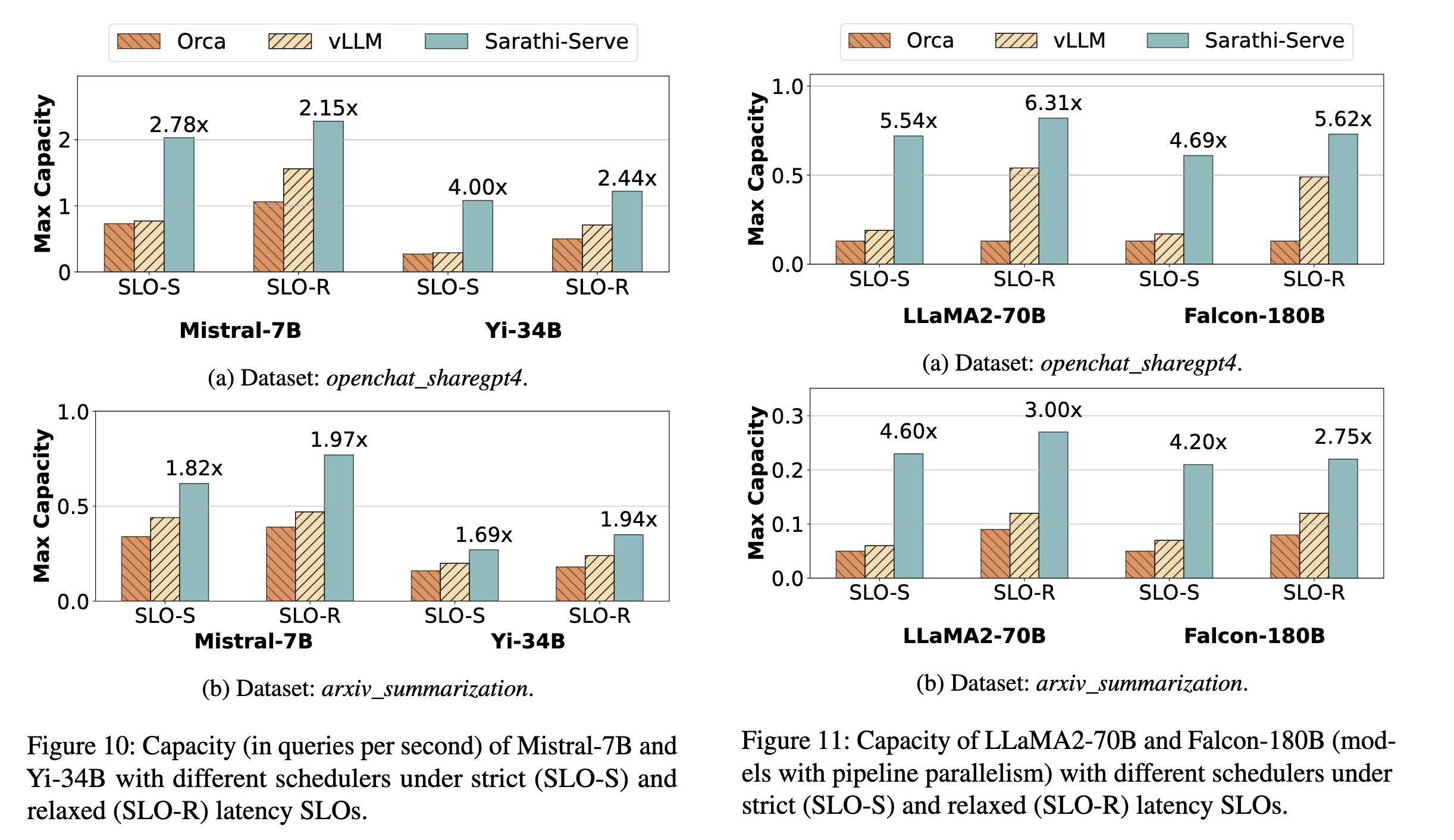
_{Figure 21. Under SLO-constrained serving, Sarathi-Serve improves serving capacity across models and setups.^[1]}

As a result of what we have talked about so far, Sarathi-Serve consistently improves serving capacity across models, with gains of about 2.6× to 5.6× depending on the model and parallelism, under realistic workloads.

Unlike benchmarks in some previous papers, Sarathi-Serve specifically measured throughput gains under SLOs, which I found interesting.

Code Example: nano-vLLM-v1#

I found a great minimal example of Chunked Prefill implied to code in https://github.com/slwang-ustc/nano-vllm-v1, a V1 version on top of nano-vllm.

    def schedule(self) -> tuple[list[Sequence], bool]:
        # ...
        token_budget = self.max_num_batched_tokens

        # schedule from the running queue
        req_index = 0
        while req_index < len(self.running) and token_budget > 0:
            seq = self.running[req_index]
            num_new_tokens = len(seq) - seq.num_cached_tokens
            if self.enable_chunked:
                # chunked prefill
                num_new_tokens = min(num_new_tokens, token_budget)
            # only allow num_new_tokens + num_cached_tokens
            # <= max model length - 1 tokens
            num_new_tokens = min(
                num_new_tokens, self.max_model_len - 1 - seq.num_cached_tokens
            )
            assert num_new_tokens > 0
            while True:
                if self.block_manager.can_append(seq, num_new_tokens):
                    seq.num_new_tokens = num_new_tokens
                    self.block_manager.may_append(seq)
                    break
                preempted_seq = self.running.pop()
                self.preempt(preempted_seq)
                # used as flag (if not preempted, we check
                # for waiting queues as well)
                preempted_seqs.append(preempted_seq)
                if len(self.running) == req_index:
                    break
            if len(self.running) == req_index:
                break
            scheduled_running_seqs.append(seq)
            token_budget -= seq.num_new_tokens
            req_index += 1

As seen in the code, instead of checking if the whole num_new_tokens for prefill requests, we also consider the token budget, which is the capacity of maximum tokens that can run in the batch. If the prefill request length is 100 tokens but we only have 20 tokens left before token budget reaches 0, we chunk the first 20 tokens and process it.

References#

1. Agrawal et al., "Taming Throughput-Latency Tradeoff in LLM Inference with Sarathi-Serve." Link
2. He, "Making Deep Learning Go Brrrr From First Principles." Link
3. Agrawal, "Sarathi-Serve" OSDI '24 Slides. Link
4. BentoML, "LLM Inference Metrics." Link
5. Choi et al., "Splitwise: Efficient Generative LLM Inference Using Phase Splitting." Link
6. Agrawal et al., "Taming Throughput-Latency Tradeoff in LLM Inference with Sarathi-Serve." Link
7. Yu et al., "Orca: A Distributed Serving System for Transformer-Based Generative Models." Link
8. UvA DL Notebooks, "Pipeline Parallelism." Link
9. Weng, "How to Train Really Large Models on Many GPUs." Link
10. Rao, "Distributed and Efficient Finetuning." Link
11. "Improving LLM Inference with Continuous Batching: Orca through tinyorca." Link
12. "Introduction to LLM Inference Part 1." Link